 Zain Baquar is an experienced data scientist and machine learning engineer. He’s Lead Technical Consultant at HSO, and has developed numerous machine learning pipelines and solutions. Prior to his role at HSO, Zain was Senior Software Engineer at Visionet Systems Inc.
In this practical step-by-step guide, Zain explains how to successfully perform time series forecasting with PyTorch. He outlines how to prepare your time series data, and takes us through the entire process with examples, from sequencing and model architecture, through to model training and inference:
Believe it or not, humans are constantly predicting things passively – even the most minuscule or seemingly trivial things. When crossing the road, we forecast where the cars will be to cross the road safely, or we try to predict exactly where a ball will be when we try to catch it. We don’t need to know the exact velocity of the car or the precise wind direction affecting the ball in order to perform these tasks – they come more or less naturally and obviously to us. These abilities are tuned by a handful of events, which over years of experience and practice allow us to navigate the unpredictable reality we live in. Where we fail in this regard, is when there are simply too many factors to take into consideration when we are actively predicting a large-scale phenomenon, like the weather or how the economy will perform one year down the line.
This is where the power of computing comes into focus – to fill the gap of our inability to take even the most seemingly random of occurrences and relate them to a future event. As we all know, computers are extremely good at doing a specific task over numerous iterations – which we can leverage in order to predict the future.
A time series is any quantifiable metric or event that takes place over a period of time. As trivial as this sounds, almost anything can be thought of as a time series. Your average heart rate per hour over a month or the daily closing value of a stock over a year or the number of vehicle accidents in a certain city per week over a year. Recording this information over any uniform period of time is considered as a time series. The astute would note that for each of these examples, there is a frequency (daily, weekly, hourly etc) of the event and a length of time (a month, year, day etc) over which the event takes place.
For a time series, the metric is recorded with a uniform frequency throughout the length of time over which we are observing the metric. In other words, the time in between each record should be the same.
In this tutorial, we will explore how to use past data in the form of a time series to forecast what may happen in the future.
The objective of the algorithm is to be able to take in a sequence of values, and predict the next value in the sequence. The simplest way to do this is to use an Auto-Regressive model, however, this has been covered extensively by other authors, and so we will focus on a more deep learning approach to this problem, using recurrent neural networks.
Let’s have a look at a sample time series. The plot below shows some data on the price of oil from 2013 to 2018.


Many machine learning models perform much better on normalised data. The standard way to normalise data is to transform it such that for each column, the mean is 0 and the standard deviation is 1. The code below provides a way to do this using the scikit-learn library.

We also want to ensure that our data has a uniform frequency – in this example, we have the price of oil on each day across these five years, so this works out nicely. If, for your data, this is not the case, Pandas has a few different ways to resample your data to fit a uniform frequency.
Once this is achieved, we are going to use the time series and generate clips, or sequences of fixed length. While recording these sequences, we will also record the value that occurred right after that sequence. For example: let’s say we have a sequence: [1, 2, 3, 4, 5, 6].
By choosing a sequence length of 3, we can generate the following sequences, and their associated targets:
[Sequence]: Target
[1, 2, 3] → 4
[2, 3, 4] → 5
[3, 4, 5] → 6
Another way to look at this is that we are defining how many steps back to look in order to predict the next value. We will call this value the training window and the number of values to predict, the prediction window . In this example, these are 3 and 1 respectively. The function below details how this is accomplished.
PyTorch requires us to store our data in a Dataset class in the following way:

We can then use a PyTorch DataLoader to iterate through the data. The benefit of using a DataLoader is that it handles batching and shuffling internally, so we don’t have to worry about implementing it for ourselves.
The training batches are finally ready after the following code:

At each iteration the DataLoader will yield 16 (batch size) sequences with their associated targets which we will pass into the model.
The class below defines this architecture in PyTorch . We’ll be using a single LSTM layer, followed by some dense layers for the regressive part of the model with dropout layers in between them. The model will output a single value for each training input.


This class is a plug n’ play Python class that I built to be able to dynamically build a neural network (of this type) of any size, based on the parameters we choose – so feel free to tune the parameters n_hidden and n_deep_players to add or remove parameters from your model. More parameters means more model complexity and longer training times, so be sure to refer to your usecase for what’s best for your data.
As an arbitrary selection, let’s create a Long ShortTerm Memory model with 5 fully connected layers with 50 neurons each, ending with a single output value for each training example in each batch. Here, sequence_ len refers to the training window and nout defines how many steps to predict; setting sequence_len as 180 and nout as 1, means that the model will look at 180 days (half a year) back to predict what will happen tomorrow.

With our model defined, we can choose our loss function and optimiser, set our learning rate and number of epochs, and begin our training loop. Since this is a regressive problem (i.e. we are trying to predict a continuous value), a safe choice is Mean Squared Error for the loss function. This provides a robust way to calculate the error between the actual values and what the model predicts. This is given by:

The optimiser object stores and calculates all the gradients needed for back propagation.

Here’s the training loop. In each training iteration, we will calculate the loss on both the training and validation sets we created earlier:


Now that the model is trained, we can evaluate our predictions.
Here we will simply call our trained model to predict on our un-shuffled data and see how different the predictions are from the true observations.


Normalised Predicted vs Actual price of oil historically. Image by author.
For a first try, our predictions don’t look too bad! And it helps that our validation loss is as low as our training loss, showing that we did not overfit the model and thus, the model can be considered to generalise well – which is important for any predictive system.
With a somewhat decent estimator for the price of oil with respect to time in this time period, let’s see if we can use it to forecast what lies ahead.
If we define history as the series until the moment of the forecast, the algorithm is simple:
1. Get the latest valid sequence from the history (of training window length).
2. Input that latest sequence to the model and predict the next value.
3. Append the predicted value on to the history.
4. Repeat from step 1 for any number of iterations.
One caveat here is that depending on the parameters chosen upon training the model, the further out you forecast, the more the model succumbs to it’s own biases and starts to predict the mean value. So we don’t want to always predict too far ahead if unnecessary, as it takes away from the accuracy of the forecast.
This is implemented in the following functions:


Let’s try a few cases.
Let’s forecast from different places in the middle of the series so we can compare the forecast to what actually happened. The way we have coded the forecaster, we can forecast from anywhere and for any reasonable number of steps. The red line shows the forecast. Keep in mind, the plots show the normalised prices on the y-axis.
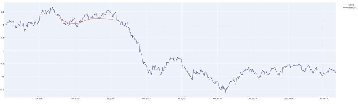
Forecasting 200 days from Q3 2013. Image by author.
Forecasting 200 days from EOY 2014/15. Image by author.

Forecasting 200 days from Q1 2016. Image by author.

Forecasting 200 days from the last day of the data. Image by author
And this was just the first model configuration we tried! Experimenting more with the architecture and implementation would definitely allow your model to train better and forecast more accurately.
There we have it! A model that can predict what will happen next in a univariate time series. It’s pretty cool when thinking about all the ways and places in which this can be applied. Yes, this article only handled univariate timeseries, in which there is a single sequence of values. However there are ways to use multiple series measuring different things together to make predictions. This is called multivariate time series forecasting, it mainly just needs a few tweaks to the model architecture which I will cover in a future article.
The true magic of this kind of forecasting model is in the LSTM layer of the model, and how it handles and remembers sequences as a recurrent layer of the neural network.
